Relationship Between the VIX and SP500 Revisited

A recent post on Bloomberg website entitled Rising VIX Paints Doubt on S&P 500 Rally pointed out an interesting observation:

While the S&P 500 Index rose to an all-time high for a second day, the advance was accompanied by a gain in an options-derived gauge of trader stress that usually moves in the opposite direction

The article refers to a well-known phenomenon that under normal market conditions, the VIX and SP500 indices are negatively correlated, i.e. they tend to move in the opposite direction. However, when the market is nervous or in a panic mode, the VIX/SP500 relationship can break down, and the indices start to move out of whack.

In this post we revisit the relationship between the SP500 and VIX indices and attempt to quantify their dislocation.  Knowing the SP500/VIX relationship and the frequency of dislocation will help options traders to better hedge their portfolios and ES/VX futures arbitrageurs to spot opportunities.

We first investigate the correlation between the SP500 daily returns and change in the VIX index [1]. The graph below depicts the daily changes in VIX as a function of SP500 daily returns from 1990 to 2016.

Volatility index and S&P500 index correaltion
Daily point change in VIX v.s. SP500 return

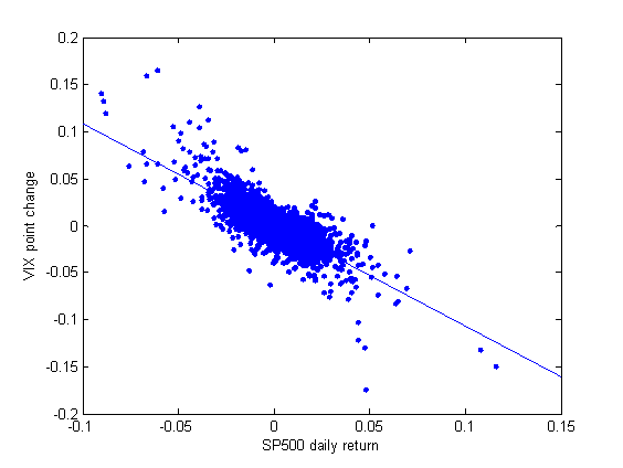
We observe that there is a high degree of correlation between the daily SP500 returns and daily changes in the VIX. We calculated the correlation and it is -0.79 [2].

We next attempt to quantify the SP500/VIX dislocation. To do so, we calculated the residuals. The graph below shows the residuals from January to December 2016.

residuals VIX/SP500 regression
Residuals of VIX/SP500

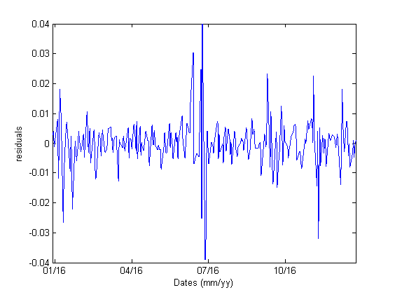
Under normal market conditions, the residuals are small, reflecting the fact that SPX and VIX are highly (and negatively) correlated, and they often move in lockstep. However, under a market stress or nervous condition, SPX and VIX can get out of line and the residuals become large.

We counted the percentage of occurrences where the absolute values of the residuals exceed 1% and 2% respectively. Table below summarizes the results

Threshold Percentage of Occurrences
1% 17.6%
2% 3.9%

We observe that the absolute values of SP500/VIX residuals exceed 1% about 17.6% of the time. This means that a delta-neutral options portfolio will experience a daily PnL fluctuation in the order of magnitude of 1 vega about 17% of the time, i.e. about 14 times per year.  The dislocation occurs not infrequently.

The Table also shows that divergence greater than 2% occurs less frequently, about 3.8% of the time. This year, 2% dislocation happened during the January selloff,  Brexit and the US presidential election.

Most of the time this kind of divergence is unpredictable. It can lead to a marked-to-market loss which can force the trader out of his position and realize the loss. So the key in managing an options portfolio is to construct positions such that if a divergence occurs, then the loss is limited and within the allowable limit.


Footnotes:

[1] We note that under different contexts, the percentage change in VIX can be used in a correlation study.  In this post, however, we choose to use the change in the VIX as measured by daily point difference. We do so because the change in VIX can be related directly to Vega PnL of an options portfolio.

[2]  The scope of this post is not to study the predictability of the linear regression model, but to estimate the frequency of SP500/VIX divergence.  Therefore, we applied linear regression to the whole data set from 1990 to 2016. For more accurate hedges, traders should use shorter time periods with frequent recalibration.

Volatility Trading Strategies, a Comparison of Volatility Risk Premium and Roll Yield Strategies

Volatility trading strategies

In previous posts, we presented 2 volatility trading strategies: one strategy is based on the volatility risk premium (VRP) and the other on the volatility term structure, or roll yield (RY).  In this post we present a detailed comparison of these 2 strategies and analyze their recent performance.

The first strategy (VRP) is based on the volatility risk premium.  The trading rules are as follows [1]:

Buy (or Cover) VXX  if VIX index <= 5D average of 10D HV of SP500

Sell (or Short) VXX  if VIX index > 5D average of 10D HV of SP500

The second strategy (RY) is based on the contango/backwardation state of the volatility term structure. The trading rules are as follows:

Buy (or Cover) VXX if 5-Day Moving Average of VIX/VXV >=1 (i.e. backwardation)

Sell (or Short) VXX if 5-Day Moving Average of  VIX/VXV  < 1 (i.e. contango)

Table below presents the backtested results from January 2009 to December 2016. The starting capital is $10000 and is fully invested in each trade (different position sizing scheme will yield different ending values for the portfolios. But the percentage return of each trade remains the same)

RY VRP
Initial capital 10000 10000
Ending capital 179297.46 323309.02
Net Profit 169297.46 313309.02
Net Profit % 1692.97% 3133.09%
Exposure % 99.47% 99.19%
Net Risk Adjusted Return % 1702.07% 3158.54%
Annual Return % 44.22% 55.43%
Risk Adjusted Return % 44.46% 55.88%
Max. system % drawdown -50.07% -79.47%
Number of trades trades 32 55
Winners 15 (46.88 %) 38 (69.09 %)

We observe that RY produced less trades, has a lower annualized return, but less drawdown than VRP. The graph below depicts the portfolio equities for the 2 strategies.

volatility risk premium and roll yield strategies
Portfolio equity for the VRP and RY strategies

It is seen from the graph that VRP suffered a big loss during the selloff of Aug 2015, while RY performed much better. In the next section we will investigate the reasons behind the drawdown.

Performance during August 2015

The graph below depicts the 10-day HV of SP500 (blue solid line), its 5-day moving average (blue dashed line), the VIX index (red solid line) and its 5-day moving average (red dashed line) during July and August 2015. As we can see, an entry signal to go short was generated on July 21 (red arrow). The trade stayed short until an exit signal was triggered on Aug 31 (blue arrow).  The system exited the trade with a large loss.

volatility risk premium relative value arbitrage
10-day Historical Volatility and VIX

The reason why the system stayed in the trade while SP500 was going down is that during that period, the VIX was always higher than 5D MA of 10D HV.  This means that 10D HV was not a good approximate for the actual volatility during this highly volatile period. Recall that the expectation value of the future realized volatility is not observable. This drawdown provides a clear example that estimating actual volatility is not a trivial task.

By contrast, the RY strategy was more responsive to the change in market condition. It went long during the Aug selloff (blue arrow in the graph below) and exited the trade with a gain. The responsiveness is due to the fact that both VIX and VXV used to generate trading signals are observable. The graph below shows VIX/VXV ratio (black line) and its 5D moving average (red line).

volatility term structure relative value arbitrage
VIX/VXV ratio


In summary, we prefer the RY strategy because of its responsiveness and lower drawdown. Both variables used in this strategy are observable. The VRP, despite being based on a good ground, suffers from a drawback that one of its variables is not observable. To improve it, one should come up with a better estimate for the expectation value of the future realized volatility.  This task is, however, not trivial.

References

[1] T Cooper, Easy Volatility Investing, SSRN, 2013