A Volatility Skew Based Trading Strategy

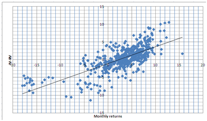
In previous blog posts, we explored the possibility of using various volatility indices in designing market timing systems for trading VIX-related ETFs. The system logic relies mostly on the persistent risk premia in the options market. Recall that there are 3 major types of risk premium:

1-Implied/realized volatilities (IV/RV)

2-Term structure

3-Skew

A summary of the systems developed based on the first 2 risk premia was published in this post.

In this article, we will attempt to build a trading system based on the third type of risk premium: volatility skew. As a measure of the volatility skew, we use the CBOE SKEW index.

According to the CBOE website, the SKEW index is calculated as follows,

The CBOE SKEW Index (“SKEW”) is an index derived from the price of S&P 500 tail risk. Similar to VIX®, the price of S&P 500 tail risk is calculated from the prices of S&P 500 out-of-the-money options. SKEW typically ranges from 100 to 150. A SKEW value of 100 means that the perceived distribution of S&P 500 log-returns is normal, and the probability of outlier returns is therefore negligible. As SKEW rises above 100, the left tail of the S&P 500 distribution acquires more weight, and the probabilities of outlier returns become more significant. One can estimate these probabilities from the value of SKEW. Since an increase in perceived tail risk increases the relative demand for low strike puts, increases in SKEW also correspond to an overall steepening of the curve of implied volatilities, familiar to option traders as the “skew”.

Our system’s rules are as follows:

Buy (or Cover) VXX if SKEW >= 10D average of SKEW

Sell (or Short) VXX if SKEW < 10D average of SKEW

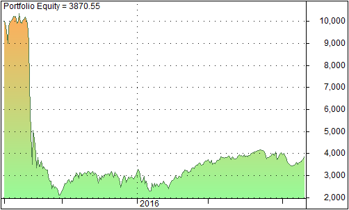
The table below summarizes important statistics of the trading system

Initial capital	10000
Ending capital	40877.91
Net Profit	30877.91
Net Profit %	308.78%
Exposure %	99.50%
Net Risk Adjusted Return %	310.34%
Annual Return %	19.56%
Risk Adjusted Return %	19.66%
Max. system % drawdown	-76.00%
Number of trades	538
Winners	285 (52.97 %)

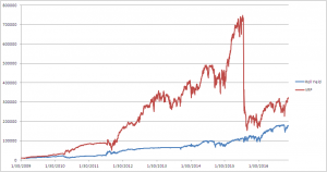
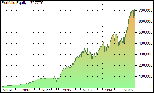
The graph below shows the equity line from February 2009 to December 2016

Portfolio equity for the volatility SKEW trading strategy

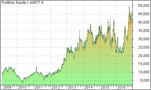
We observe that this system does not perform well as the other 2 systems [1]. A possible explanation for the weak performance is that VXX and other similar ETFs’ prices are affected more directly by the IV/RV relationship and the term structure than by the volatility skew. Hence using the volatility skew as a timing mechanism is not as accurate as other volatility indices.

In summary, the system based on the CBOE SKEW is not as robust as the VRP and RY systems. Therefore we will not add it to our existing portfolio of trading strategies.

Footnotes

[1] We also tested various combinations of this system and results lead to the same conclusion.

Relationship Between the VIX and SP500 Revisited

A recent post on Bloomberg website entitled Rising VIX Paints Doubt on S&P 500 Rally pointed out an interesting observation:

While the S&P 500 Index rose to an all-time high for a second day, the advance was accompanied by a gain in an options-derived gauge of trader stress that usually moves in the opposite direction

The article refers to a well-known phenomenon that under normal market conditions, the VIX and SP500 indices are negatively correlated, i.e. they tend to move in the opposite direction. However, when the market is nervous or in a panic mode, the VIX/SP500 relationship can break down, and the indices start to move out of whack.

In this post we revisit the relationship between the SP500 and VIX indices and attempt to quantify their dislocation. Knowing the SP500/VIX relationship and the frequency of dislocation will help options traders to better hedge their portfolios and ES/VX futures arbitrageurs to spot opportunities.

We first investigate the correlation between the SP500 daily returns and change in the VIX index [1]. The graph below depicts the daily changes in VIX as a function of SP500 daily returns from 1990 to 2016.

Volatility index and S&P500 index correaltion — Daily point change in VIX v.s. SP500 return

We observe that there is a high degree of correlation between the daily SP500 returns and daily changes in the VIX. We calculated the correlation and it is -0.79 [2].

We next attempt to quantify the SP500/VIX dislocation. To do so, we calculated the residuals. The graph below shows the residuals from January to December 2016.

residuals VIX/SP500 regression — Residuals of VIX/SP500

Under normal market conditions, the residuals are small, reflecting the fact that SPX and VIX are highly (and negatively) correlated, and they often move in lockstep. However, under a market stress or nervous condition, SPX and VIX can get out of line and the residuals become large.

We counted the percentage of occurrences where the absolute values of the residuals exceed 1% and 2% respectively. Table below summarizes the results

Threshold	Percentage of Occurrences
1%	17.6%
2%	3.9%

We observe that the absolute values of SP500/VIX residuals exceed 1% about 17.6% of the time. This means that a delta-neutral options portfolio will experience a daily PnL fluctuation in the order of magnitude of 1 vega about 17% of the time, i.e. about 14 times per year. The dislocation occurs not infrequently.

The Table also shows that divergence greater than 2% occurs less frequently, about 3.8% of the time. This year, 2% dislocation happened during the January selloff, Brexit and the US presidential election.

Most of the time this kind of divergence is unpredictable. It can lead to a marked-to-market loss which can force the trader out of his position and realize the loss. So the key in managing an options portfolio is to construct positions such that if a divergence occurs, then the loss is limited and within the allowable limit.

Footnotes:

[1] We note that under different contexts, the percentage change in VIX can be used in a correlation study. In this post, however, we choose to use the change in the VIX as measured by daily point difference. We do so because the change in VIX can be related directly to Vega PnL of an options portfolio.

[2] The scope of this post is not to study the predictability of the linear regression model, but to estimate the frequency of SP500/VIX divergence. Therefore, we applied linear regression to the whole data set from 1990 to 2016. For more accurate hedges, traders should use shorter time periods with frequent recalibration.

Volatility Trading Strategies, a Comparison of Volatility Risk Premium and Roll Yield Strategies

Volatility trading strategies

In previous posts, we presented 2 volatility trading strategies: one strategy is based on the volatility risk premium (VRP) and the other on the volatility term structure, or roll yield (RY). In this post we present a detailed comparison of these 2 strategies and analyze their recent performance.

The first strategy (VRP) is based on the volatility risk premium. The trading rules are as follows [1]:

Buy (or Cover) VXX if VIX index <= 5D average of 10D HV of SP500

Sell (or Short) VXX if VIX index > 5D average of 10D HV of SP500

The second strategy (RY) is based on the contango/backwardation state of the volatility term structure. The trading rules are as follows:

Buy (or Cover) VXX if 5-Day Moving Average of VIX/VXV >=1 (i.e. backwardation)

Sell (or Short) VXX if 5-Day Moving Average of VIX/VXV < 1 (i.e. contango)

Table below presents the backtested results from January 2009 to December 2016. The starting capital is $10000 and is fully invested in each trade (different position sizing scheme will yield different ending values for the portfolios. But the percentage return of each trade remains the same)

	RY	VRP
Initial capital	10000	10000
Ending capital	179297.46	323309.02
Net Profit	169297.46	313309.02
Net Profit %	1692.97%	3133.09%
Exposure %	99.47%	99.19%
Net Risk Adjusted Return %	1702.07%	3158.54%
Annual Return %	44.22%	55.43%
Risk Adjusted Return %	44.46%	55.88%
Max. system % drawdown	-50.07%	-79.47%
Number of trades trades	32	55
Winners	15 (46.88 %)	38 (69.09 %)

We observe that RY produced less trades, has a lower annualized return, but less drawdown than VRP. The graph below depicts the portfolio equities for the 2 strategies.

volatility risk premium and roll yield strategies — Portfolio equity for the VRP and RY strategies

It is seen from the graph that VRP suffered a big loss during the selloff of Aug 2015, while RY performed much better. In the next section we will investigate the reasons behind the drawdown.

Performance during August 2015

The graph below depicts the 10-day HV of SP500 (blue solid line), its 5-day moving average (blue dashed line), the VIX index (red solid line) and its 5-day moving average (red dashed line) during July and August 2015. As we can see, an entry signal to go short was generated on July 21 (red arrow). The trade stayed short until an exit signal was triggered on Aug 31 (blue arrow). The system exited the trade with a large loss.

volatility risk premium relative value arbitrage — 10-day Historical Volatility and VIX

The reason why the system stayed in the trade while SP500 was going down is that during that period, the VIX was always higher than 5D MA of 10D HV. This means that 10D HV was not a good approximate for the actual volatility during this highly volatile period. Recall that the expectation value of the future realized volatility is not observable. This drawdown provides a clear example that estimating actual volatility is not a trivial task.

By contrast, the RY strategy was more responsive to the change in market condition. It went long during the Aug selloff (blue arrow in the graph below) and exited the trade with a gain. The responsiveness is due to the fact that both VIX and VXV used to generate trading signals are observable. The graph below shows VIX/VXV ratio (black line) and its 5D moving average (red line).

volatility term structure relative value arbitrage — VIX/VXV ratio

In summary, we prefer the RY strategy because of its responsiveness and lower drawdown. Both variables used in this strategy are observable. The VRP, despite being based on a good ground, suffers from a drawback that one of its variables is not observable. To improve it, one should come up with a better estimate for the expectation value of the future realized volatility. This task is, however, not trivial.

References

[1] T Cooper, Easy Volatility Investing, SSRN, 2013

October was Favorable for Short Volatility Strategies

Last month was particularly favorable for short volatility strategies. In this post, we will investigate the reasons behind it.

First, the main PnL driver of a delta neutral, short gamma and short vega strategy is the spread between the implied volatility (IV) and the subsequently realized volatility (RV) of returns. Trading strategies such as long butterfly is profitable when, during the life of the position, RV is low compared to IV. The graph below shows the difference between IV and RV for SP500 during the last 5 months. (Note that RV is shifted by 1 month, so that IV-RV presents accurately the spread between the implied volatility and the volatility realized during the following month). As we can see from the graph, IV-RV was high, around 4%-7%, during October (the area around the “10/16” mark). Hence short volatility strategies were generally profitable during October.

implied minus realized volatilities — IV-RV spreads of SP500

The second reason for the profitability is more subtle. The graph below shows the IV-RV spreads in function of monthly returns. As we can see, there is a high degree of correlation between IV-RV and the monthly returns. In fact, we calculated the correlation for the last 10 years and it is 0.69

IV-RV spreads v.s. SP500 monthly returns

This means that when IV-RV is high, SP500 usually trends up. This was the case, for example, during the month after Brexit (see the area around the “07/16” mark on the first graph). However, when the market trends, the cost of hedging in order to keep the position delta neutral is high. By contrast, even though IV-RV was high in October, the market moved in a range, thus helping us to minimize our hedging costs. This factor therefore contributed to the profitability of short volatility strategies.

In summary, October was favorable for short volatility strategies due to the high IV-RV spread and the range bound nature of the market.

A Volatility Term Structure Based Trading Strategy

In previous 2 articles, we explored a volatility trading strategy based on the volatility risk premium (VRP). The strategy performed well up until August 2015, and then it suffered a big loss during the August selloff.

In this article, we explore another volatility trading strategy, also discussed in Ref [1]. This strategy is based on the volatility term structure [2].

It is well known that volatilities exhibit a term structure which is similar to the yield curve in the interest rate market. The picture below depicts the volatility term structure for SP500 as at August 31 2016 [3].

volatility term structure trading strategy — SP500 Volatility Term Structure at Aug 31 2016

Most of the time the term structure is in contango. This means that the back months have higher implied volatilities than the front months. However, during a market stress, the volatility term structure curve usually inverts. In this case we say that the volatility term structure curve is in backwardation (a similar phenomenon exists in the interest rate market which is called inversion of the yield curve).

The basic idea of the trading strategy is to use the state (contango/backwardation) of the volatility term structure as a timing mechanism. Specifically, we go long if the volatility term structure is in backwardation and go short otherwise. To measure the slope of the term structure, we use the VIX and VXV volatility indices which represent the 1M and 3M implied volatilities of SP500 respectively.

The trading rules are as follows,

Buy (or Cover) VXX if 5-Day Moving Average of VIX/VXV >=1 (i.e. backwardation)

Sell (or Short) VXX if 5-Day Moving Average of VIX/VXV < 1 (i.e. contango)

The Table below presents the results

	All trades	Long trades	Short trades
Initial capital	10000	10000	10000
Ending capital	177387.15	19232.01	168155.15
Net Profit	167387.15	9232.01	158155.15
Net Profit %	1673.87%	92.32%	1581.55%
Exposure %	99.44%	6.64%	92.80%
Net Risk Adjusted Return %	1683.22%	1390.38%	1704.17%
Annual Return %	46.07%	9.00%	45.05%
Risk Adjusted Return %	46.33%	135.54%	48.54%

All trades	30	15 (50.00 %)	15 (50.00 %)
Avg. Profit/Loss	5579.57	615.47	10543.68
Avg. Profit/Loss %	13.29%	2.29%	24.28%
Avg. Bars Held	64.53	9.8	119.27

Winners	14 (46.67 %)	4 (13.33 %)	10 (33.33 %)
Total Profit	208153.11	36602.85	171550.26
Avg. Profit	14868.08	9150.71	17155.03
Avg. Profit %	36.58%	25.17%	41.14%
Avg. Bars Held	129.64	14.25	175.8
Max. Consecutive	3	1	4
Largest win	71040.59	18703.17	71040.59
# bars in largest win	157	35	157

Losers	16 (53.33 %)	11 (36.67 %)	5 (16.67 %)
Total Loss	-40765.96	-27370.84	-13395.12
Avg. Loss	-2547.87	-2488.26	-2679.02
Avg. Loss %	-7.09%	-6.02%	-9.45%
Avg. Bars Held	7.56	8.18	6.2
Max. Consecutive	5	6	2
Largest loss	-9062.89	-8222.29	-9062.89
# bars in largest loss	6	8	6

Max. trade drawdown	-28211.89	-15668.21	-28211.89
Max. trade % drawdown	-23.97%	-18.20%	-23.97%
Max. system drawdown	-32794.28	-26555.13	-37915.18
Max. system % drawdown	-50.07%	-90.85%	-34.31%
Recovery Factor	5.1	0.35	4.17
CAR/MaxDD	0.92	0.1	1.31
RAR/MaxDD	0.93	1.49	1.41
Profit Factor	5.11	1.34	12.81
Payoff Ratio	5.84	3.68	6.4
Standard Error	12109.91	6401.13	12526.9
Risk-Reward Ratio	1.49	0.15	1.36
Ulcer Index	11.25	42.48	8.24
Ulcer Performance Index	3.62	0.08	4.81
Sharpe Ratio of trades	0.8	0.53	0.97
K-Ratio	0.0745	0.0073	0.0683

The graph below shows the portfolio equity from 2009 up to August 2016.

The annual rerun is 46% and the drawdown is 50%. There are 2 interesting observations

This strategy did not suffer a large loss like the VRP strategy during the August selloff of last year
Long volatility trades are profitable

In the next installment we will compare the 2 strategies, volatility risk premium and roll yield, in details.

References

[1] T Cooper, Easy Volatility Investing, SSRN, 2013

[2] Note that there is a so-called term structure risk premium in the options market that is not often discussed in the literature. The strategy discussed in this post, however, is not meant to exploit the term structure risk premium. It uses the term structure as a timing mechanism.

[3] The volatility term structure presented here is calculated based on VIX futures, which are the expectation values of 30-day forward implied volatility. Therefore, it is theoretically different from the term structure of spot volatilities which are calculated from SP500 options. Practically speaking, the 2 volatility term structures are highly correlated, and we use the futures curve in this article for illustration purposes.

Volatility Trading Strategy, a System Based on Volatility Risk Premium

Last year, we presented backtested results for a VXX trading strategy. The system’s logic is based upon the concept of volatility risk premium. In short, the trading rules are as follows:

Buy (or Cover) VXX if 5D average of (VIX index -10D HV of SP500) < 0

Sell (or Short) VXX if 5D average of (VIX index -10D HV of SP500)>0

The strategy performed well in backtest. In this follow-up post, we look at how it has performed since last year. The Table below summarizes the results

	All trades	Long trades	Short trades
Initial capital	10000	10000	10000
Ending capital	3870.55	9095.02	4775.53
Net Profit	-6129.45	-904.98	-5224.47
Net Profit %	-61.29%	-9.05%	-52.24%
Exposure %	100.00%	14.67%	85.33%
Net Risk Adjusted Return %	-61.29%	-61.68%	-61.23%
Annual Return %	-60.50%	-8.86%	-51.48%
Risk Adjusted Return %	-60.50%	-60.42%	-60.33%

All trades	11	5 (45.45 %)	6 (54.55 %)
Avg. Profit/Loss	-557.22	-181	-870.74
Avg. Profit/Loss %	-3.35%	-4.40%	-2.47%
Avg. Bars Held	24.55	8.6	37.83

Winners	6 (54.55 %)	2 (18.18 %)	4 (36.36 %)
Total Profit	2366.97	365.38	2001.59
Avg. Profit	394.49	182.69	500.4
Avg. Profit %	13.75%	6.46%	17.40%
Avg. Bars Held	32.5	7.5	45
Max. Consecutive	2	2	2
Largest win	1308.08	239.26	1308.08
# bars in largest win	102	8	102

Losers	5 (45.45 %)	3 (27.27 %)	2 (18.18 %)
Total Loss	-8496.42	-1270.36	-7226.06
Avg. Loss	-1699.28	-423.45	-3613.03
Avg. Loss %	-23.87%	-11.64%	-42.21%
Avg. Bars Held	15	9.33	23.5
Max. Consecutive	2	2	1
Largest loss	-6656.33	-625.51	-6656.33
# bars in largest loss	29	11	29

The strategy produced 11 trades with 6 trades (55%) being winners. However, it suffered a big loss during August. The graph below shows the portfolio equity since last August.

quantitative trading volatility — VRP volatility trading strategy

Large losses are typical of short volatility strategies. An interesting observation is that after the large drawdown, the strategy has recovered, as depicted by the upward trending equity line after August. This is usually the case for short volatility strategies.

Despite the big loss, the overall return (not shown) is still positive. This means that the strategy has a positive expectancy. Drawdown can be minimized by using a correct position size, stop losses, and a good portfolio allocation scheme. Another solution is to construct limited-loss positions using VXX options.

Volatility Trading through VIX ETFs

It is well known that persistent biases exist in various markets. For example, in the tennis market, there exists a longshot bias. Similarly, financial markets exhibit a persistent bias called the risk premium. Formally, the risk premium is defined as

where E_Q denotes the expectation value of X, a stochastic variable, in the risk-neutral world, and E_P denotes the expectation value of X in the real world. X can be, for example, commodity prices, FX rates, etc. See reference 1 for a thorough discussion of various risk premia in financial markets.

Of our particular interest is the case where X is the realized volatility (RV) of a stock or stock index. The risk premium in this case is often called volatility (or variance) risk premium (VRP). If we substitute X in the above equation with the RV of SP500, then E_Q (RV) becomes the VIX index, and the VRP becomes VIX- E_P (RV).

Traders often try to exploit the VRP by trading listed options or OTC variance swaps. Another way to harvest the VRP is through trading VIX -based Exchange Trade Funds such as VXX. In this post we explore the latter possibility.

The most difficult problem when designing a VRP-based trading strategy is that E_P(RV), which is needed in order to calculate the VRP, is not observable. The best we can do is to use a quantitative method to estimate it.

Reference 2 tested various forms of E_P(RV) estimate: GARCH, historical volatilities (HV). The author found that 10-day HV is the most effective. They then further smoothed out the HV by using a 5-day moving average in order to avoid whipsaws. The trading rules are as follows:

Buy (or Cover) VXX if VIX index <= 5D average of 10D HV of SP500

Sell (or Short) VXX if VIX index > 5D average of 10D HV of SP500

The Table below summarizes the trading strategy’s statistics. The starting capital is $10000. It is fully invested in each trade

	All trades	Long trades	Short trades
Initial capital	10000	10000	10000
Ending capital	727774.91	-74688.89	812463.8
Net Profit	717774.91	-84688.89	802463.8
Net Profit %	7177.75%	-846.89%	8024.64%
Exposure %	99.02%	6.58%	92.44%
Net Risk Adjusted Return %	7248.42%	-12868.01%	8680.57%
Annual Return %	93.38%	N/A	96.68%
Risk Adjusted Return %	94.29%	N/A	104.58%

All trades	43	21 (48.84 %)	22 (51.16 %)
Avg. Profit/Loss	16692.44	-4032.8	36475.63
Avg. Profit/Loss %	12.04%	2.34%	21.29%
Avg. Bars Held	38.79	6.14	69.95

Winners	32 (74.42 %)	12 (27.91 %)	20 (46.51 %)
Total Profit	918340.82	94671.52	823669.31
Avg. Profit	28698.15	7889.29	41183.47
Avg. Profit %	18.13%	8.45%	23.93%
Avg. Bars Held	47.47	5.92	72.4
Max. Consecutive	9	5	8
Largest win	198505.33	36704.45	198505.33
# bars in largest win	78	7	78

Losers	11 (25.58 %)	9 (20.93 %)	2 (4.65 %)
Total Loss	-200565.92	-179360.41	-21205.5
Avg. Loss	-18233.27	-19928.93	-10602.75
Avg. Loss %	-5.69%	-5.82%	-5.10%
Avg. Bars Held	13.55	6.44	45.5
Max. Consecutive	3	4	1
Largest loss	-38701.76	-38701.76	-16516.3
# bars in largest loss	4	4	41
Max. trade drawdown	-300537.33	-38701.76	-300537.33
Max. trade % drawdown	-46.12%	-12.49%	-46.12%
Max. system drawdown	-331363.27	-164250.75	-300537.33
Max. system % drawdown	-52.21%	-95.16%	-64.93%
Recovery Factor	2.17	-0.52	2.67
CAR/MaxDD	1.79	N/A	1.49
RAR/MaxDD	1.81	N/A	1.61
Profit Factor	4.58	0.53	38.84
Payoff Ratio	1.57	0.4	3.88
Standard Error	56932.62	32093.21	72795.73
Risk-Reward Ratio	1.67	-0.46	1.51
Ulcer Index	12.97	111.97	11.45
Ulcer Performance Index	6.78	N/A	7.97
Sharpe Ratio of trades	1.46	1.36	1.71
K-Ratio	0.0775	-0.0214	0.07

We observe that the short trades are profitable while the long ones lost money. The CARG is 93.4%, which is high, but so is the drawdown of -52%. The graph below shows the portfolio equity

Volatility portfolio equity — VRP Volatility Trading Strategy

In summary, the VRP can be harvested through VIX ETF. However the drawdown is high. This strategy is viable if it is part of an asset allocation scheme. It would enhance the portfolio risk-adjusted return if we allocate, for example, 10% of our portfolio to this strategy, and the rest to equity and fixed income investments.

References

[1 ] A. Ilmanen, Expected Returns: An Investor’s Guide to Harvesting Market Rewards, John Wiley & Sons , 2011

[2] T Cooper, Easy Volatility Investing, SSRN, 2013

Pricing Convertible Bonds-An Example

In the previous post, we outlined the main steps in pricing a convertible bond using the Binomial Tree approach. In this follow-up post, we provide a hypothetical example of a straight convertible bond.

The specifics of the hypothetical convertible bond are as follows,

INPUTS
Stock price	100
Volatility	0.25
Risk Free Rate	0.02
Risky Rate (risk free+credit spread)	0.08
Coupon	0.06
Maturity (in years)	5
Conversion ratio	10

Using the formula provided in the previous post, we calculated the up and down moves, and probability of the up move. The results are

MODEL PARAMETERS
dt	1.00
u	1.28
d	0.78
Probability Up	0.48

Once the tree parameters are calculated, we next build the tree, and then work backward from the end nodes in order to obtain the convertible bond’s price at time zero. As the final result, the bond price is $1319 (per $1000 notional)

To see the details of the calculations of the tree, follow the instruction at the bottom of this page. Note that this is a simplified example. In real life, convertible bonds are usually more complex. They often include features such as call, put, contingency conversion options. The call and put options can be implemented using the formula given in the previous post.

I hope that this and previous posts demystified a little bit the complexities of convertible bonds. Let us know if you have any questions.

Follow this link for more derivative pricing models in Excel

Pricing Convertible Bonds and Preferred Shares

A convertible bond (or preferred share) is a hybrid security, part debt and part equity. Its valuation is derived from both the level of interest rates and the price of the underlying equity. Several modeling approaches are available to value these complex hybrid securities such as Binomial Tree, Partial Differential Equation and Monte Carlo simulation. One of the earliest pricing convertible bond approaches was the Binomial Tree model originally developed by Goldman Sachs [1,2] and this model allows for an efficient implementation with high accuracy. The Binomial Tree model is flexible enough to support the implementation of bespoke exotic features such as redemption and conversion by the issuer, lockout periods, conversion and retraction by the share owner etc.

In this post, we will summarize the key steps in pricing convertible bond method using the Binomial Tree approach. Detailed description of the method and examples are provided in references [1,2].

Generally, the value of a convertible bond with embedded features depends on:

The underlying common stock price
Volatility of the common stock
Dividend yield on the common stock
The risk free interest rate
The credit worthiness of the preferred share issuer

Within the binomial tree framework, the common stock price at each node is described as

pricing convertible bond

where S₀ is the stock price at the valuation date; u and d are the up and down jump magnitudes. The superscript j refers to the time step and i to the jump. The up and down moves are calculated as

and

where is the stock volatility, and is the time step.

The risk neutral probability of the up move, u, is

and the probability the down move is 1-p

After building a binomial tree for the common stock price, the convertible bond price is then determined by starting at the end of the stock price tree where the payoff is known with certainty and going backward until the time zero (valuation date). At each node, Pj,i the value of the convertible is

where m denotes the conversion ratio.

If the bond is callable, the payoff at each node is

The payoff of a putable bond is

Here C and P are the call and put values respectively; r denotes the risk-free rate.

The above equations are the key algorithms in the binomial tree approach. However, there are several considerations that should be addressed due to the complexities of the derivative features

Credit spreads (credit risk) of the issuers which usually are not constant.
Interest rates can be stochastic.
Discount rate ri,j depends on the conversion probability at each node. This is due to the fact that when the common share price is well below the strike, the preferred share behaves like a corporate bond and hence we need to discount with a risky curve. If the share is well above the strike then the preferred behaves like a common stock and the riskless curve need to be used.
The notice period: the issuer tends to call the bond if the stock price is far enough above the conversion price such that a move below it is unlikely during the notice period. For most accurate results, the valuation would require a call adjustment factor. This factor is empirical and its value could be determined by calibration to stock historical data.

This approach in pricing convertible bond can be implemented in scripting languages such as VBA and Matlab. In the next installment, we will provide a concrete example of pricing a convertible bond. If you have a convertible bond that you want us to use as example, send it to us.

References

[1] Valuing Convertible Bonds as Derivatives, Quantitative Strategies Research Notes, Goldman Sachs, November 1994.

[2] Pricing Convertible Bonds, Kevin B. Connolly, Wiley, 1998.

Brazil Beats Germany

The World Cup is over and Germany won the much coveted trophy. This World Cup will be remembered for its beautiful attacking-style games as well as one of the most crushing defeats in football history: the Host lost 1-7 to Germany in the semi final.

However, the Brazilians do not have to wait for another 4 years in order to have a chance to revenge against Germany. Their stock market has already beaten the German’s one. The chart below shows the ratio of the Brazil ETF (EWZ) v.s. Germany ETF (EWG) and we can see that the ratio is in an uptrend.

Statistically, the Brazilian market has underperformed over the last 3 years. It lost -29%, while the German market gained 45%. However, EWZ started bouncing at the beginning of this year from an oversold condition.

The bounce is also supported by fundamental factors: Brazil is an exporter of commodities and the uptrend in base metals lends support to its market recovery. Additionally, the upcoming Summer Olympics in Rio in 2016 will give a boost to the local economy.

Germany, on the other hand, is suffering from problems in Europe: deflation threat, a weak euro, negative interest rates, geopolitical tension in Ukraine and Russia, and a possible bank failure in Portugal, just to name a few. This is a good opportunity for pair traders who want to take advantage of the divergence.