Volatility of Gold Pairs

It is commonly believed that commodity pairs are relatively easy to trade because their underlying stocks are pegged to a certain commodity market. Sometimes, however, this is not the case.

Gold stock pairs have been difficult to trade lately. One of the economic reasons is that as the gold spot declines, it approaches the production cost of around $1200 per ounce, and a small change in the spot would induce a big change (in percentage terms) in the profit margin of the producer. In other words, a small change in the spot would make a larger impact on the company’s profit and loss, thus causing a bigger fluctuation in the stock price. The big fluctuation magnifies the fundamental discrepancies inherent in the stocks of the pair. Consequently, deviations from the norm are likely due to more fundamental than statistical reasons. For quantitative traders who rely solely on statistics to make decision, it has been more difficult trading gold pairs profitably.

We can look at this problem from the options pricing theoretic point of view.  The average production cost of $1200 per ounce can be considered a put option strike. If gold spot deeps below $1200, then the stock is considered in the money. Since late 2012 the “options” are near at the money, and gold stocks behave more or less like ATM options that have greater gamma risks.

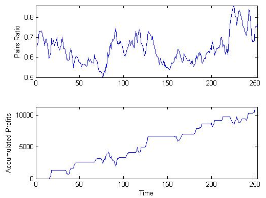
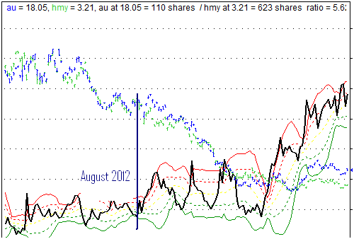
In the chart below, the solid black line shows the ratio of two gold stocks, AngloGold Ashanti (AU) v.s. Harmony Gold Mining (HMY). As it can be seen, starting August 2012 (marked with the blue vertical line), the declining in the stock prices started accelerating, and the oscillation in the pair ratio started increasing accordingly. Put it differently, the gamma has caused a greater oscillation in the pair ratio.

In the future, if gold spot trends up, the “options” will get out of the money, and the gamma risk will decrease. In this case gold stock pairs are expected to behave more regularly, thus providing better trade opportunities for statistical arbitrage traders.

Why Do Arbitrage Opportunities Still Exist?

A question arbitrageurs are frequently asked is “why aren’t the pricing inefficiencies arbitraged away?”  This is a very legitimate question.

I believe that in some areas of trading and investment, the number of arbitrage opportunity is diminishing. Take, for example, statistical arbitrage; its profitability is decreasing due to the increasing popularity of the method, competition among traders and advancement in information technology. In other areas of trading, opportunities still exist and persist. For example, in option trading, the volatility risk premium seems to persist despite the fact that it has become widely known.  Here are some possible explanations for the persistence of the volatility risk premium:

  • Due to regulatory pressures, banks have to meet Value-at-Risk requirements and prevent shortfalls. Therefore, they buy out-of-money puts, or OTC variance swaps to hedge the tail risks.
  • Asset management firms that want to guarantee a minimum performance and maintain a good Sharpe ratio must buy protective puts.
  • The favorite long-shot bias plays a role in inflating the prices of the puts.
  • There might be some utility effects that the traditional option pricing models are not capable of taking into account.
  • There are difficulties in implementing and executing an investment strategy that exploits the volatility risk premium and that is at the same time within the limits of margin requirements and drawdown tolerance.

We believe, however, that with a good understanding of the sources of cheapness and expensiveness of volatility, a sensible trading plan can be worked out to exploit the volatility risk premium within reasonable risk limits. We love to hear your suggestion.

Current Implied Volatility is Cheap

The phenomenon of the favorite long-shot bias (or volatility risk premium) can be exploited in order to construct a profitable options trading strategy. Basically, such a strategy would consist of selling overpriced options and hedging the risks using cheaper (or more precisely less overpriced) options. As can be seen from the graph below, the implied volatility (IV, yellow line) is generally higher than the historical volatility (HV, blue line). However, as of late, IV deepened below HV, which is rather unusual. A premium selling strategy in this kind of volatility environment might still profitable. However, the risks will likely outweigh the rewards.

The cheapness of IV is also confirmed by the volatility cone. As can be seen below, at the money IV, (depicted in white diamonds) is below the current HV (depicted by the white line).

A long volatility trade will have a higher probability of success in this kind of market.

The Favorite Long-shot Bias in Option Markets

The favorite long-shot bias is a phenomenon that has been studied extensively in gambling markets. A question has arisen naturally: does this bias exist in financial markets?

In a paper entitled “The Favorite /Long-shot Bias in S&P 500 and FTSE 100 Index Futures Options: The Return to Bets and the Cost of Insurance”, Hodges, Tompkins and Ziemba examined whether the favorite/long-shot bias that has been found in gambling markets (particularly in horse racing markets) applies to options markets. The motivation came from the fact that puts and calls on stock index futures represent leveraged short or long positions on the index and their behavior might have similar features to racetrack bets.

The authors found that both call and put options on the S&P 500 (and FTSE 100 to some degree) with one and three months to expiration display a relationship between probabilities of finishing in the money and expected returns that is very similar to the favorite long-shot bias in horse racing markets. In another word, they found evidence that was consistent with the hypothesis that investors tend to overpay for put options as the expected cost of insurance and call options as low-cost, high-payoff gambles.

This finding is consistent with results published by other researchers under the general framework of the volatility risk premium which refers to the fact that implied volatility in equity index options often tends to overstate realized volatility. In fact, the favorite/long-shot bias provides an alternative explanation for the existence of volatility risk premium.

For practitioners, a question arose: how to structure a position that takes advantage of the favorite long-shot bias?

Another BRIC in the Wall

A good reward/risk trade is a one where fundamentals and technicals are aligned. We have seen two fundamentally similar countries (Canada/Australia) but they did not make a good pair for short-term trading. We have also seen two seemingly different economies (Australia/Indonesia) but that made a good pair.

There exist, however, some pairs that have good technical and fundamental relationships. India (INDL) and Russia (RUSL) are two emerging markets; they are part of the BRIC countries. The ratio chart (upper panel, below) exhibits a regular oscillating pattern, albeit somewhat volatile. The backtested equity line (lower panel) is, however, orderly upward.

Backtest results showed a winning percentage of 88% and a profit factor of 1.86, so this is a good pair to trade. As a bonus, these stocks are leveraged ETFs, hence the pair is also suitable for intra-day scalping.


Quantitative Poker Player

If there were an equivalent of a quantitative trader in the poker world, then Chris Ferguson would be a perfect example. Chris earned a PhD in computer science in the late nineties and went on to become a professional poker player and gambling and lottery industry consultant.  He has won five World Series of Poker events, including the 2000 WSOP Main Event, and the 2008 NBC National Heads-Up Poker Championship. His playing style is highly mathematical as he uses a strong knowledge of game theory and has developed computer simulations to improve his understanding of the game.  Last but not least, Chris also tried his hands at day trading.

I watched a video of him being interviewed by Michael Covel, who is known as one of the original Turtles. Although the video is short, it successfully brings across the following important points:

  • Play with the best players and learn from them.
  • Spend more time away from the tables doing analysis, thus developing an analytical thought process.
  • Do not focus on last hands’ results. Winning or losing does not matter in the short run. Focus on the process and long-term results.
  • Put faith in mathematics. Try to make decisions less emotional as possible and mathematical as much as possible.
  • Study the game hard. Analyze the game from mathematical stand points.
  • Practice and practice and practice.

Although Chris discussed these points in order to educate aspiring professional poker players, they are definitely important lessons for quantitative traders as well.

Longshot Bias in Tennis Market

The longshot bias is an observed phenomenon in sports betting where on average bettors tend to overvalue (undervalue) “long shots” and undervalue (overvalue) the favorites. It has been studied extensively in betting markets such as horse racing, American football, ice hockey and soccer. The most plausible explanation is provided by behavior finance which studies the betting patterns of several types of bettors: informed, uninformed, amateur, professional using advanced models such as utility function theory. The tennis market, however, attracted much less attention, and very little research was conducted in this area.

Unlike other sports, the tennis market presents some particularities, mostly:

  • The cost of becoming an “informed” bettor is relatively low. Hence there is no uninformed, “fun” bettor who just enjoys an outing at the courts as they often do in horse racing,
  • Insider information is less valuable because almost everything (e.g. players’ injuries) is visible and disseminated quickly to the public,
  • Unlike team sports, tennis does not have a large number of fan clubs with permanent and fervent allegiance. Therefore the prices (odds) are less likely to be distorted by supporters’ sentiment,
  • The transaction cost is low.

Among noteworthy articles, the one published by D. Forest and I. McHale, entitled “Longshot bias, insight from the betting on men’s professional tennis”, presented interesting results regarding the longshot bias in the tennis market.  Using publicly available data, the authors tabulated returns of strategies that bet on favorites and underdogs from January 2001 to April 2004. They demonstrated that:

  • Betting on underdogs yielded statistically significant losses,
  • Betting on favorites was break-even in 2001 and made positive returns in 2002-04.

From their results, it was concluded that men’s tennis market is weak form inefficient, and a positive longshot bias exists. Therefore good values are found by betting on strong favorites. Bettors should use this result in developing their strategies.

Sports Arbitrage

Although sport and financial markets are seemingly two different worlds, arbitrage trading and sports betting have a lot in common. Trading strategies and risk-management techniques used in financial markets can be applied to sports betting and vice versa. As in financial markets, pricing inefficiencies do exist in the sport bookmaking markets which result in opportunities for arbitrageurs.

Sports arbitrage can be loosely categorized into two main types:

  • Inter-bookmaker arbitrage which exploits bookmakers’ different opinions on sport events’ outcomes or plain pricing errors.
  • Intra-bookmaker arbitrage which exploits the relative mispricing, based on the actual and implied odds, of a sport event.

Of the two types of sports arbitrage, the latter is being used by us. It is in a sense very similar to the options volatility trading strategy where one seeks an edge by taking advantage of the discrepancy between historical and implied volatilities of an underlying asset. To see how sports arbitrage work, let’s go through a real-life example.

Soccer is unarguably one of the most popular sports in the world. At the club level, UEFA Champions League is the most prestigious competition for a European soccer club. The final this year will be held on May 25 at the Wembley stadium. As of this writing there are four clubs remain in the competition, two from Germany and two from Spain. The draw for the semi-finals was held last Friday and the following match up will occur:

Bayern Munich – Barcelona        

Borussia Dortmund – Real Madrid

The first leg of the Bayern Munich- Barcelona match will be played on April 23 in Bayern’s homeland. As of this writing, the implied probability of a Bayern Munich win is 40%. It is calculated from the posted odds of 2.5 on Ladbrokes, a well-known bookmaker.

Note, however, that this price is not static; it can vary from now until the end of the match, thus creating short-term trading opportunities.  The actual probability of winning for Bayern Munich, calculated based on its past and recent performance, is 45.9% (2.18 in decimal form).  Consequently, there is an opportunity for arbitrage. If we place a bet on Ladbrokes now, we’ll have an edge of 5.9 %.

As can be seen from the example above, the goal of sports arbitrage is to find as many as possible this kind of mispricing opportunity and repeat the betting process over and over again. This way we play a positive expectation game and will make money in the long run.

Relative Pricing

Many popular trading strategies are based on some forms of fundamental or technical analysis. They attempt to value securities based on some fundamental multiples or technical indicators. These valuation techniques can be considered “absolute pricing”. Arbitrage trading strategies, on the other hand, are based on a so-called relative pricing. So what is relative pricing?

The theory and practice of relative pricing are derived from the principle of no arbitrage. Stephen A. Ross, a renowned professor of finance, is known for saying:

You can make even a parrot into a learned political economist—all he must learn are the two words “supply” and “demand”… To make the parrot into a learned financial economist, he only needs to learn the single word “arbitrage”.

What he was referring to is what financial economists call the principle of no risk-free arbitrage or the law of one price which states that: “Any two securities with identical future payouts, no matter how the future turns out, should have identical current prices.”

Relative pricing based on the principle of no risk-free arbitrage underlies most of the derivative pricing models in quantitative finance. That is, a security is valued based on the prices of other securities that are as similar to it as possible. For example an over-the-counter interest-rate swap is valued based on the prices of other traded swaps and not on, for example, some macro-economic factors. A bespoke basket option is valued based on the prices of its components’ vanilla options.

The principle of no risk-free arbitrage is employed in its original form in trading strategies such as convertible and volatility arbitrage. In statistical arbitrage  it is, however, relaxed; it normally involves stocks  which are similar but not 100% identical.

In summary, relative pricing based on the principle of no risk-free arbitrage is very different from absolute pricing. It is the foundation of many derivative pricing models and quantitative trading strategies.

Correlation Decreasing

Statistical arbitrage trading relies on, among other factors, the correlation between stocks. It is important to note, however, that correlation, like volatility, is not static, but time dependent and changing. Different market condition has a different level of correlation, and this has an important implication for stat-arb trading PnL.

We have been in a bull market lately, and it’s fairly common in bull markets for correlations to relax. The chart below depicts the CBOE Implied Correlation Index for SP500 stocks from November 2011 to March 2013. As we can see from the graph, the correlation is in a downtrend; it decreased from 80 % in Dec 2011 to about 55% in early March 2013.

The decrease in correlation explains in part why we have observed lots of dislocated pair relationships lately.  This dislocation increased the likelihood of pair divergence, hence one should exercise more caution when choosing pairs.