
In a previous post, we discussed how the dynamics of assets are priced in the options prices. We recently came across a newly published article [1] that explored the same topic but from a different perspective that does not involve options.
The conclusion of the new article [1] is consistent with the previous one [2]; that is, the volatilities of mean-reverting assets are smaller than those of assets that follow the GBM process. The reverse applies to trending assets.
In this post, we are going to investigate whether the mean-reverting/trending property of an asset has any impact on a trading strategy’s PnL volatility.
To do this, we first generate asset prices using Monte Carlo simulations. We evolve the asset prices in both mean-reverting and trending regimes for 500 days. We then apply a simple trading system to the simulated asset prices. The trading system is as follows,
Go LONG when the Relative Strength Index <40, SHORT when the Relative Strength Index >70
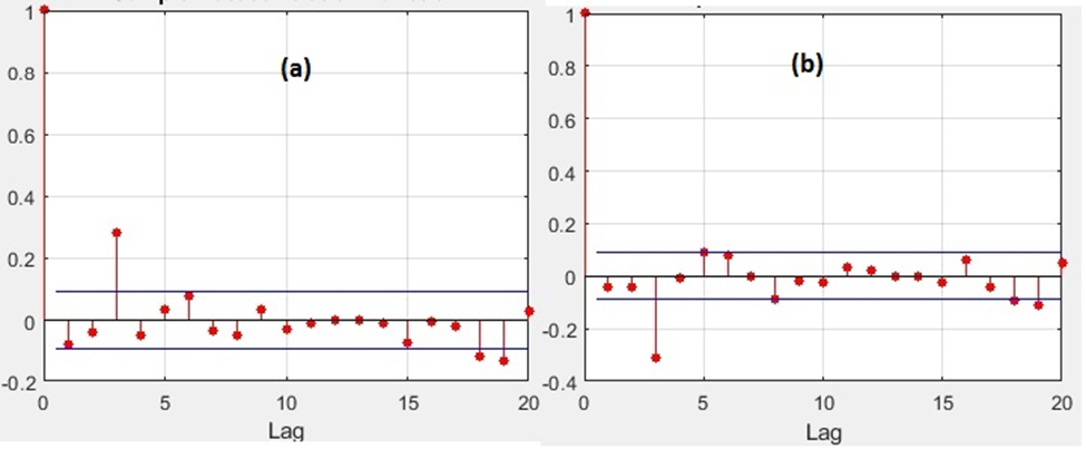
The picture below shows the Autocorrelation Functions (ACF) of the asset returns. Panels (a) and (b) present ACFs of the trending and mean-reverting assets respectively. It’s clear that the assets are trending and mean-reverting at lag 3, respectively.
The picture below shows the simulated equity curves of the trading strategy applied to the trending (a) and mean-reverting (b) assets. The starting capital is $100 in both cases.
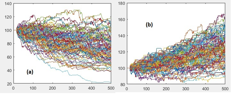
Visually, we do not observe any difference in terms of PnL dispersion. Indeed, the standard deviation of the terminal wealth at day 500 is $18.9 in the case of the trending asset (a), and $17.3 in the case of the mean-reverting asset (b). Is the difference statistically significant? We don’t think so.
This numerical experiment shows that the PnL volatility of a trading strategy has little to do with the underlying asset’ mean-reverting/trending property. Maybe it depends more on the strategy itself? (Note that in this example, we utilize a mean-reverting strategy). What would happen at the portfolio level?
References
[1] L. Middleton, J. Dodd, S. Rijavec, Trading styles and long-run variance of asset prices, 2021, arXiv:2109.08242
[2] Liao, S.L. and Chen, C.C. (2006), The valuation of European options when asset returns are autocorrelated, Journal of Futures Markets, 26, 85-102.