In this post, I will continue exploring various aspects of the volatility index and the associated volatility futures.
Data
To conduct this study, data is essential. Below are the data sources:
- Spot VIX: Yahoo Finance provides data but no longer allows direct downloads. With some programming, a workaround can be found, but the most convenient option is to use Barchart.
https://www.barchart.com/stocks/quotes/$VIX/price-history/historical
- VX Futures: CBOE offers historical data in CSV format.
https://www.cboe.com/us/futures/market_statistics/historical_data/
- Short-Term Futures Index:
While not directly utilized in this issue, I use this data to validate other ideas. For completeness, here is the download link:
https://www.spglobal.com/spdji/en/indices/indicators/sp-500-vix-short-term-index-mcap/#overview
Statistics for spot VIX and VX Futures
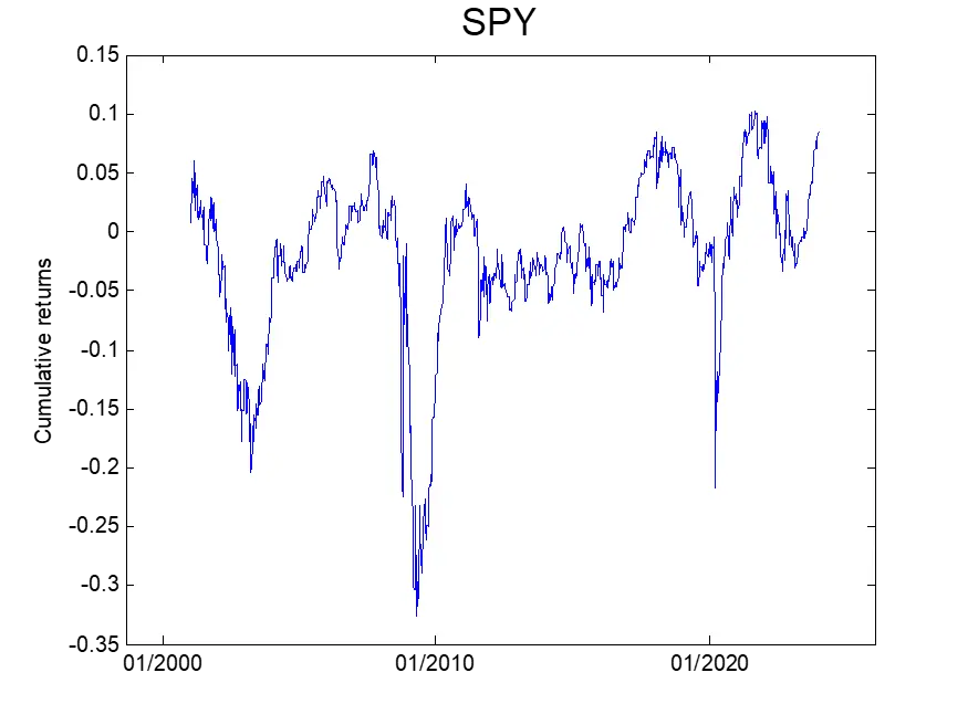
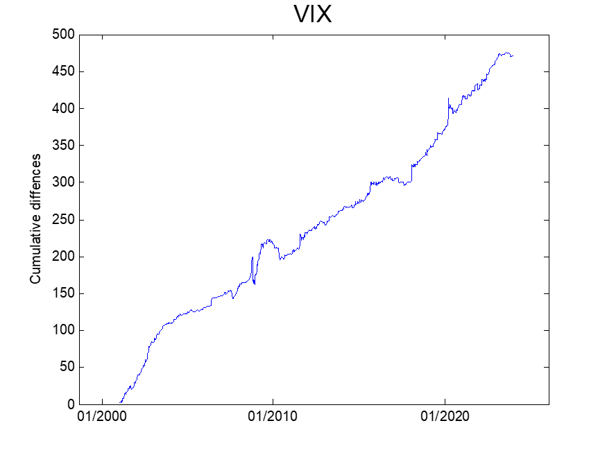
The table below provides statistics for the S&P 500 (tracked by SPY), spot VIX, and VX futures. It shows the percentage of days the S&P 500 index is up and the percentage of days VX futures are in contango, where the front-month futures price is lower than the next-month futures price.
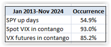
From January 2013 to November 2024, the S&P 500 index was up 54.9% of the time, while VX futures were in contango most of the time (85.2%).
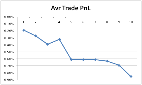
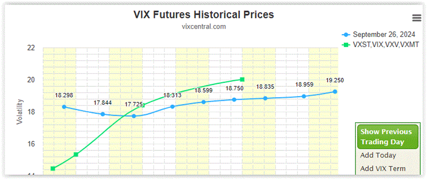
The next table presents the number of days VX futures were in backwardation while the spot VIX was in contango. Spot VIX in contango is defined as the 1M spot VIX being less than the 3M spot VIX.
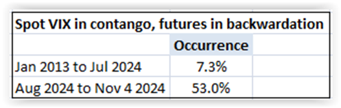
From January 2013 to July 2024, this situation was very rare, occurring only 7% of the time. However, from August 1 to November 4, 2024, this divergence occurred with much higher frequency, 53% of the time.
This situation presented a high reward/risk trade opportunity. For instance, one could structure a trade to capitalize on the high likelihood of VX futures returning to contango and a decline in the overall volatility level. One potential trade is buying a put option in VXX. We’ll discuss this strategy in an upcoming webinar.
Seasonality of Volatility
With the holiday season approaching, the equity world often discusses the “Santa Rally.” This raises the question: Is there any seasonality in the volatility market?
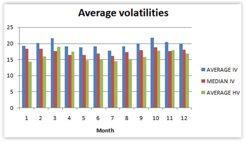
The graph below shows the average and median monthly implied and historical volatilities. A clear seasonal pattern is observed, with low volatility between April and July and high volatility in October. However, for December, there is no discernable pattern—volatility can be either high or low during this period.
Educational Video
This webinar by Prof Andrew Papanicolaou covers fundamental concepts of VX futures, such as contango, backwardation, and roll yield. It also presents an approach to modeling the VX futures term structure.
Abstract:
We study VSTOXX, VSTOXX futures and VSTOXX exchange-traded notes (ETNs) econometrically. We find that different rates of mean reversion capture fluctuations in the short and long maturities, respectively. We fit an exponential Ornstein-Uhlenbeck (OU) model to the data and find it to capable of simulating ETN time series that have similar properties to the historical observed ETN time series. We compare these results to a similar study performed on ETNs and futures for VIX. We also look at the joint behavior of VIX and VSTOXX futures, and explore portfolio allocation strategies among ETNs for both markets.
Closing Thoughts
The volatility market offers unique insights and opportunities for investors. By understanding concepts like contango, backwardation, and seasonality, we can structure strategies with favorable risk-reward profiles.
Let me know your thoughts in the comments below.
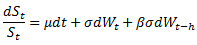
 and in case β=0 the price dynamics becomes GBM.