A lot of research has been devoted to answering the question: do options price in the volatility risks correctly? The most noteworthy phenomenon (or bias) is called the volatility risk premium, i.e. options implied volatilities tend to overestimate future realized volatilities. Much less attention is paid, however, to the underlying asset dynamics, i.e. to answering the question: do options price in the asset dynamics correctly?
Note that within the usual BSM framework, the underlying asset is assumed to follow a GBM process. So to answer the above question, it’d be useful to use a different process to model the asset price.
We found an interesting article on this subject [1]. Instead of using GBM, the authors used a process where the asset returns are auto-correlated and then developed a closed-form formula to price the options. Specifically, they assumed that the underlying asset follows an MA(1) process,
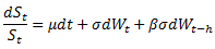
where β represents the impact of past shocks and h is a small constant. We note that  and in case β=0 the price dynamics becomes GBM.
After applying some standard pricing techniques, a closed-form option pricing formula is derived which is similar to BSM except that the variance (and volatility) contains the autocorrelation coefficient,
![]()
From the above equation, it can be seen that
- When the underlying asset is mean reverting, i.e. β<0, which is often the case for equity indices, the MA(1) volatility becomes smaller. Therefore if we use BSM with σ as input for volatility, it will overestimate the option price.
- Conversely, when the asset is trending, i.e. β>0, BSM underestimates the option price.
- Time to maturity, τ, also affects the degree of over- underpricing. Longer-dated options will be affected more by the autocorrelation factor.
References
[1] Liao, S.L. and Chen, C.C. (2006), Journal of Futures Markets, 26, 85-102.