A convertible bond (or preferred share) is a hybrid security, part debt and part equity. Its valuation is derived from both the level of interest rates and the price of the underlying equity. Several modeling approaches are available to value these complex hybrid securities such as Binomial Tree, Partial Differential Equation and Monte Carlo simulation. One of the earliest pricing convertible bond approaches was the Binomial Tree model originally developed by Goldman Sachs [1,2] and this model allows for an efficient implementation with high accuracy. The Binomial Tree model is flexible enough to support the implementation of bespoke exotic features such as redemption and conversion by the issuer, lockout periods, conversion and retraction by the share owner etc.
In this post, we will summarize the key steps in pricing convertible bond method using the Binomial Tree approach. Detailed description of the method and examples are provided in references [1,2].
Generally, the value of a convertible bond with embedded features depends on:
- The underlying common stock price
- Volatility of the common stock
- Dividend yield on the common stock
- The risk free interest rate
- The credit worthiness of the preferred share issuer
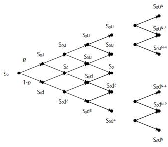
Within the binomial tree framework, the common stock price at each node is described as


where S0 is the stock price at the valuation date; u and d are the up and down jump magnitudes. The superscript j refers to the time step and i to the jump. The up and down moves are calculated as

and

where  is the stock volatility, and
  is the time step.
The risk neutral probability of the up move, u, is

and the probability the down move is 1-p
After building a binomial tree for the common stock price, the convertible bond price is then determined by starting at the end of the stock price tree where the payoff is known with certainty and going backward until the time zero (valuation date). At each node, Pj,i the value of the convertible is

where m denotes the conversion ratio.
If the bond is callable, the payoff at each node is

The payoff of a putable bond is

Here C and P are the call and put values respectively; r denotes the risk-free rate.
The above equations are the key algorithms in the binomial tree approach. However, there are several considerations that should be addressed due to the complexities of the derivative features
- Credit spreads (credit risk) of the issuers which usually are not constant.
- Interest rates can be stochastic.
- Discount rate ri,j depends on the conversion probability at each node. This is due to the fact that when the common share price is well below the strike, the preferred share behaves like a corporate bond and hence we need to discount with a risky curve. If the share is well above the strike then the preferred behaves like a common stock and the riskless curve need to be used.
- The notice period: the issuer tends to call the bond if the stock price is far enough above the conversion price such that a move below it is unlikely during the notice period. For most accurate results, the valuation would require a call adjustment factor. This factor is empirical and its value could be determined by calibration to stock historical data.
This approach in pricing convertible bond can be implemented in scripting languages such as VBA and Matlab. In the next installment, we will provide a concrete example of pricing a convertible bond. If you have a convertible bond that you want us to use as example, send it to us.
References
[1] Valuing Convertible Bonds as Derivatives, Quantitative Strategies Research Notes, Goldman Sachs, November 1994.
[2] Pricing Convertible Bonds, Kevin B. Connolly, Wiley, 1998.
