Category: convertible bonds

In the previous post, we outlined the main steps in pricing a convertible bond using the Binomial Tree approach. In this follow-up post, we provide a hypothetical example of a straight convertible bond.

The specifics of the hypothetical convertible bond are as follows,

INPUTS
Stock price	100
Volatility	0.25
Risk Free Rate	0.02
Risky Rate (risk free+credit spread)	0.08
Coupon	0.06
Maturity (in years)	5
Conversion ratio	10

Using the formula provided in the previous post, we calculated the up and down moves, and probability of the up move. The results are

MODEL PARAMETERS
dt	1.00
u	1.28
d	0.78
Probability Up	0.48

Once the tree parameters are calculated, we next build the tree, and then work backward from the end  nodes in order to obtain the convertible bond’s price at time zero. As the final result, the bond price is $1319 (per $1000 notional)

To see the details of the calculations of the tree, follow the instruction at the bottom of this page. Note that this is a simplified example. In real life, convertible bonds are usually more complex. They often include features such as call, put, contingency conversion options. The call and put options can be implemented using the formula given in the previous post.

I hope that this and previous posts demystified a little bit the complexities of convertible bonds. Let us know if you have any questions.

Follow this link for more derivative pricing models in Excel

A convertible bond (or preferred share) is a hybrid security, part debt and part equity. Its valuation is derived from both the level of interest rates and the price of the underlying equity. Several modeling approaches are available to value these complex hybrid securities such as Binomial Tree, Partial Differential Equation and Monte Carlo simulation. One of the earliest pricing convertible bond approaches was the Binomial Tree model originally developed by Goldman Sachs [1,2] and this model allows for an efficient implementation with high accuracy. The Binomial Tree model is flexible enough to support the implementation of bespoke exotic features such as redemption and conversion by the issuer, lockout periods, conversion and retraction by the share owner etc.

In this post, we will summarize the key steps in pricing convertible bond method using the Binomial Tree approach. Detailed description of the method and examples are provided in references [1,2].

Generally, the value of a convertible bond with embedded features depends on:

• The underlying common stock price
• Volatility of the common stock
• Dividend yield on the common stock
• The risk free interest rate
• The credit worthiness of the preferred share issuer

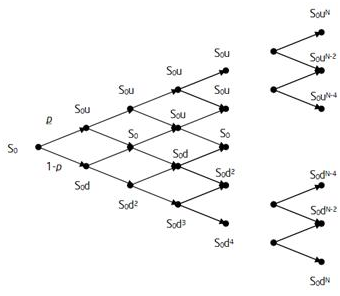
Within the binomial tree framework, the common stock price at each node is described as

where S₀ is the stock price at the valuation date; u and d are the up and down jump magnitudes. The superscript j refers to the time step and i to the jump. The up and down moves are calculated as

and

where is the stock volatility, and  is the time step.

The risk neutral probability of the up move, u, is

and the probability the down move is 1-p

After building a binomial tree for the common stock price, the convertible bond price is then determined by starting at the end of the stock price tree where the payoff is known with certainty and going backward until the time zero (valuation date). At each node, Pj,i  the value of the convertible is

where m denotes the conversion ratio.

If the bond is callable, the payoff at each node is

The payoff of a putable bond is

Here C and P are the call and put values respectively; r denotes the risk-free rate.

The above equations are the key algorithms in the binomial tree approach. However, there are several considerations that should be addressed due to the complexities of the derivative features

• Credit spreads (credit risk) of the issuers which usually are not constant.
• Interest rates can be stochastic.
• Discount rate ri,j depends on the conversion probability at each node. This is due to the fact that when the common share price is well below the strike, the preferred share behaves like a corporate bond and hence we need to discount with a risky curve. If the share is well above the strike then the preferred behaves like a common stock and the riskless curve need to be used.
• The notice period: the issuer tends to call the bond if the stock price is far enough above the conversion price such that a move below it is unlikely during the notice period. For most accurate results, the valuation would require a call adjustment factor. This factor is empirical and its value could be determined by calibration to stock historical data.

This approach in pricing convertible bond can be implemented in scripting languages such as VBA and Matlab. In the next installment, we will provide a concrete example of pricing a convertible bond. If you have a convertible bond that you want us to use as example, send it to us.

References

[1] Valuing Convertible Bonds as Derivatives, Quantitative Strategies Research Notes, Goldman Sachs, November 1994.

[2] Pricing Convertible Bonds, Kevin B. Connolly, Wiley, 1998.