
Position sizing and portfolio allocation have not received much attention in the options trading community. In this post we are going to apply a simple position sizing rule and see how it performs within the context of volatility trading.
An option position can be sized by using, for example, a Markov Model where the size of the position can be a function of the regime transition probability [1]. While this is a research venue that we would like to explore, we decided to start with a simpler approach. We chose an algorithm that is intuitive enough for both quant and non-quant portfolio managers and traders.
We utilize the market timing rule proposed by Faber [2] who applied it to different asset classes in the context of portfolio allocation. The rule is as follows
Buy when monthly price > 10M SMA (10 Month Simple Moving Average)
Sell and move to cash when monthly price < 10M SMA
This remarkably simple timing rule has been used successfully by Faber and others. It has proved to significantly improve portfolios’ risk-adjusted returns [3].
Within the context of volatility trading, we compare 2 option strategies
1-NoTiming: Sell 1-Month at-the-money (ATM) put option on every option expiration Friday. The option is held until maturity, i.e. for a month. The position is kept delta neutral, i.e. it is rehedged at the end of every day.
2-10M-SMA: Similar to the above except that Faber’s timing rule is applied, i.e. we only sell an ATM put option if the closing price of the underlying is greater than its 10M SMA. Note, however, that unlike Faber, here we define the end of month as the option expiration Friday, and not the calendar end of month.
A short discussion on the rationale for choosing a market timing rule is in order here. Within the context of portfolio allocation, the 10M SMA rule is used for timing the direction of the market, i.e. the PnL driver is mostly market beta. Our trade’s PnL driver is, on the other hand, the dynamics of the implied/realized volatility spread. But as shown in a previous post, the IV/RV volatility dynamics correlates highly with the market returns. Therefore, we thought that we could use a directional timing strategy to size an options portfolio despite the fact that their PnL drivers are different, at least theoretically.
We tested the 2 strategies on SPY options from February 2007 to November 2016. Table below provides a summary of the trade statistics (average PnLs, winning/losing trades and drawdowns are in dollar).
| Strategy | NoTiming | 10M-SMA |
| Number of Trades | 115 | 81 |
| Percent Winners | 0.68 | 0.69 |
| Average P&L | 18.84 | 14.87 |
| Largest losing trade | -269.79 | -248.50 |
| Largest winning trade | 243.54 | 154.22 |
| Profit Factor (W/L) | 1.77 | 1.64 |
| Worst drawdown | -633.24 | -339.91 |
Graph below shows the equity curves of the 2 strategies
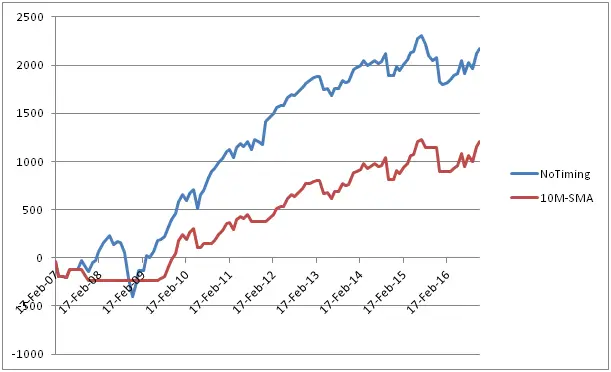
As it is observed from the Table and the Graph, except for the worst drawdown, we don’t see much of an improvement when the 10M-SMA timing rule is applied. Although the 10M-SMA strategy avoided the worst period of the Global Financial Crisis, overall it made less money than the NoTiming strategy.
The non-improvement of Faber’s rule in the context of volatility selling probably relates to the fact that we are using a directional timing algorithm to size a trade whose PnL driver is the volatility dynamics . A position sizing algorithm based directly on the volatility dynamics would have a better chance of success. We are currently extending our research in this direction; any comment, feedback is welcome.
References:
[1] C. Donninger, Timing the Tail-Risk-Protection of the SPY with VIX-Futures by a Hidden Markov Model. The Wool-Milk-Sow Strategy. April 2017, http://www.godotfinance.com/pdf/TailRiskProtectionHMM.pdf
[2] M. Faber, A Quantitative Approach to Tactical Asset Allocation, Journal of Investing , 16, 69-79, 2007
[3] See for example A. Clare, J. Seaton, P. Smith and S. Thomas, The Trend is Our Friend: Risk Parity, Momentum and Trend Following in Global Asset Allocation, Aug 2012, https://papers.ssrn.com/sol3/papers.cfm?abstract_id=2126478
How about a backtest with the same rules, but buying calls above sma 10 and out of the market below the sma 10 would be interesting to see if that makes a difference
Or the (writing)put example but with 6 month (favourable momentum period) options
Or using 6 month put credit spreads to take the volatility even more out and even scale up the leverage with the spreads because it acts as a stoploss against market crashes
Hi Kelly, I think the 10M SMA rule works better if we don’t rehedge, i.e. we take on directional risks. So your strategies will work if we just make static bets. I’ll run a test on one of them. Thanks for your suggestions
Backtesting it is better than ẗhinking”;-)
Closing out positions with written puts who go under the sma 10 have on average more implied volatility when they where opened above sma 10 .
With spreads you not only eliminate that cost but also harvest it on the wings
The OTM wing in the put spread might present an advantage if you “let the delta run”, i.e. you bet on direction. In case your bet is on the IV/RV vol spread (as it is the case in this study), i.e. you flatten out the delta at EOD, the wing can be a liability, since its price is rich due to skew and gap risk premia
The skew is in your advantage with rising volatility (situations wich can cause closing the spread ,(declining under sma 10))
When the index is rising and volatility is declining the spread will close itself by expiring worthless
If you let the delta run, which is what you’re suggesting, then adding an OTM long put might be advantageous (depending on your definition of risk-adjusted returns); if you dynamically hedge, no, especially with short-dated options
I didnt mean to dynamicly hedge just to open a spread and close it under sma 10
Or let it even expire under sma 10 and reopen above sma 10
My guess is that it will return higher sharp ratios regardless of skew , and the higher sharp ratios can leverage it also in higher absolute returns wich would be foolish with naked options to do
buying low implied vol calls above sma 10 wont have this problem either, they also have some damage control in rising implied vol to cushion directional losses
Yes, I called your strategy a static bet in my first reply, i.e. no rehedge, just open and let it run. Will run this test see how it performs. My guess is the performance will depend on maturities, as short and long dated options are priced differently
Agree re: buying call when IV is low
If you observe put write returns vs the index you will notice that after the index is below the sma 10 the put write equitycurve is initially still rising before it also starts the decline, wich makes sense because the implied vol is higher in relation to the first moment of decline of the index
Same happens when the bear trend reverses to bull, the put write equitycurve starts rising in advance of the curve of the index wich also makes sense because vol is still high in the initial stages of trend reversal.
Backtest this: dont use the sma 1o on the index but on the put write index itself it will enhance sharp AND absolute returns with put writing with sma 10 filter
Quite an interesting observation, will take a closer look. Thanks again
I feel a better way to deal with this issue is to use a delta-hedged option return, rather than raw option return.
Hi Biao, the PnL is already that of a delta-hedged option position
I am trying to reproduce your results as a learning exercise, but I guess there is some hidden part of your algorithm, because the simple writing options once per month + delta hedging doesn’t work, there is no profit. If you can send me more information which I can put it in my script, I can put it in my script, if you want something to compare with, of course. Thanks for a nice article.
Hi Pavel, the delta hedging algorithm used in this post is a standard one that you can find in any text book on options pricing theory (see e.g. John Hull). Result presented here is pretty consistent with literature on volatility risk premium. If you send me a high-level description of your algorithm through email, I can compare notes. Thanks
Hi N. Nguyen, I put some results to my blog: http://www.bluetrader.cz/delta-hedging-ano-ne/
It’s in Czech language, but you can see the pictures, there are as follows:
1. selling put once a month
2. selling put once a month, but only when ClosePrice>SMA200
3. selling put once a month, with delta hedging
4. selling put once a month, but only when ClosePrice>SMA200, with delta hedging.
I will send you the testing script details to your e-mail in a bit.
Thank you for the tip for the book, it looks very good.
Thank you Pavel
Hi,
I was wondering if you could confirm what your data source is for the options?
Thanks!
The options data is from ivolatility.com