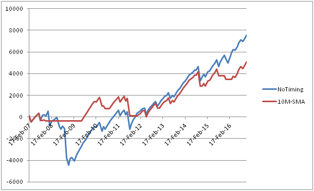
In this post, we are going to examine a trading system with the goal of using it as a hedge for long equity exposure. To this end, we test a simple, short-only momentum system. The rules are as follows,
Short at the close when Close of today < lowest Close of the last 10 days
Cover at the close when Close of today > lowest Close of the last 10 days
The Table below presents results for SPY from 1993 to the present. We performed the tests for 2 different volatility regimes: low (VIX<=20) and high (VIX>20). Note that we have tested other lookback periods and VIX filters, but obtained qualitatively the same results.
| Number of Trades | Winner | Average trade PnL | |
| All | 455 | 24.8% | -0.30% |
| VIX<=20 | 217 | 23.5% | -0.23% |
| VIX>20 | 260 | 26.5% | -0.37% |
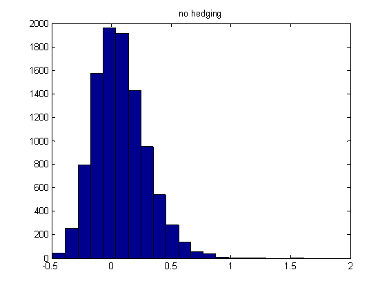
It can be seen that the average PnL for all trades is -0.3%, so overall shorting SPY is a losing trade. This is not surprising, since in the short term the SP500 exhibits a strong mean reverting behavior, and in a long term it has a positive drift.
We still expected that when volatility is high, the SP500 would exhibit some momentum characteristics and short selling would be profitable. The result indicates the opposite. When VIX>20, the average trade PnL is -0.37%, which is higher (in absolute value) than the average trade PnL for the lower volatility regime and all trades combined (-0.23% and -0.3% respectively). This result implies that the mean reversion of the SP500 is even stronger when the VIX is high.
The average trade PnL, however, does not tell the whole story. We next look at the maximum favorable excursion (MFE). Table below summarizes the results
| Average | Median | Max | |
| VIX<=20 | 0.83% | 0.44% | 10.59% |
| VIX>20 | 1.62% | 0.73% | 24.25% |
Despite the fact that the short SPY trade has a negative expectancy, both the average and median MFEs are positive. This means that the short SPY trades often have large unrealized gains before they are exited at the close. Also, as volatility increases, the average, median and largest MFEs all increase. This is consistent with the fact that higher volatility means higher risks.
The above result implies that during a sell-off, a long equity portfolio can suffer a huge drawdown before the market stabilizes and reverts. Therefore, it’s prudent to hedge long equity exposure, especially when volatility is high.
An interesting, related question arises: should we use options or futures to hedge, which one is cheaper? Based on the average trade PnL of -0.37% and gamma rent derived from the lower bound of the VIX, a back of the envelope calculation indicated that hedging using futures appears to be cheaper.