Financial models and strategies are usually universal and can be applied across different asset classes. However, in some cases, they must be adapted to the unique characteristics of the underlying asset. In this post, I’m going to discuss option pricing models and trading strategies in commodities, specifically in the crude oil market.
Volatility Smile in the Commodity Market
Paper [1] investigates the volatility smile in the crude oil market and demonstrates how it differs from the smile observed in the equity market. It proposes to use the new method developed by Carr and Wu in order to study the volatility smile of commodities. Specifically, the authors examine the volatility smile of the United States Oil ETF, USO.
Findings
– This paper examines the information derived from the no-arbitrage Carr and Wu formula within a new option pricing framework in the USO (United States Oil Fund) options market.
– The study investigates the predictability of this information in forecasting future USO returns.
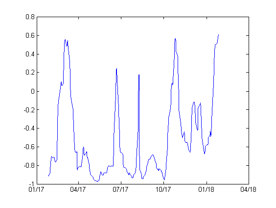
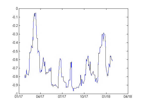
– Using the no-arbitrage formula, risk-neutral variance, and covariance estimates are obtained under the new framework.
– The research identifies the term structure and dynamics of these risk-neutral estimates.
– The findings reveal a “U”-shaped implied volatility smile with a positive curvature in the USO options market.
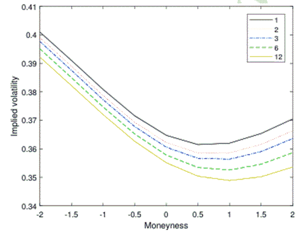
Usually, an equity index such S&P 500 exhibits a downward-sloping implied volatility pattern, i.e. a negative implied volatility skew. Oil, on the other hand, possesses a different volatility smile. This is because while equities are typically associated with crash risks, oil prices exhibit both sharp spikes and crashes, leading to a different implied volatility pattern. This highlights the importance of considering the specific characteristics and dynamics of different asset classes when analyzing and interpreting implied volatility patterns.
Reference
[1] Xiaolan Jia, Xinfeng Ruan, Jin E. Zhang, Carr and Wu’s (2020) framework in the oil ETF option market, Journal of Commodity Markets, Volume 31, September 2023, 100334
Statistical Arbitrage in the Crude Oil Markets
Reference [2] directly applies statistical arbitrage techniques, commonly used in equity markets, to the crude oil market. It utilizes cointegration to construct a statistical arbitrage portfolio. Various methods are then used to test for stationarity and mean reversion: the Quandt likelihood ratio (QLR), augmented Dickey-Fuller (ADF) test, autocorrelations, and the variance ratio. The constructed strategy performed well both in- and out-of-sample.
Findings
– This paper introduces the concept of statistical arbitrage through a trading strategy known as the mispricing portfolio.
– It focuses specifically on mean-reverting strategies designed to exploit persistent anomalies observed in financial markets.
– Empirical evidence is presented to demonstrate the effectiveness of statistical arbitrage in the crude oil markets.
– The mispricing portfolio is constructed using cointegration regression, establishing long-term pricing relationships between WTI crude oil futures and a replication portfolio composed of Brent and Dubai crude oils.
-Mispricing dynamics revert to equilibrium with predictable behaviour. Trading rules, which are commonly used in equity markets, are then applied to the crude oil market to exploit this pattern.
Reference
[2] Viviana Fanelli, Mean-Reverting Statistical Arbitrage Strategies in Crude Oil Markets, Risks 2024, 12, 106.
Closing Thoughts
As we’ve seen, techniques and models utilized in the equity market can sometimes be applied directly to the crude oil market, while other times they need to be adapted to the unique characteristics of the crude oil market. In any case, strong domain knowledge is essential.
Educational Video
In this webinar, Quantitative Trading in the Oil Market, Dr Ilia Bouchouev delivers an interesting and insightful presentation on algorithmic trading in the oil market. He also encourages viewers to apply the techniques discussed for the oil market to other markets, such as equities.
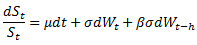
 and in case β=0 the price dynamics becomes GBM.